Practical Considerations for Antiderivative Anti-Aliasing

In audio signal processing, it is often useful to use nonlinear functions for things like saturation, wavefolding, and more. While nonlinear functions can create interesting sounds, they often create difficulty in the world of signal processing, particularly by invalidating many of the handy mathematical theorems that hold up in the world of linear signal processing. One particularly nasty issue that arises when using nonlinear functions on digital audio is aliasing.

In this article, we’ll give a brief discussion of what aliasing is, and how it is typically dealt with. Then, we’ll introduce a relatively new anti-aliasing technique called Antiderivative Anti-Aliasing (ADAA), and discuss some practical considerations for implementing various nonlinear systems with ADAA.

As usual, this article can be read with code as a Jupyter Notebook.

Aliasing

First, what is aliasing? This question brings us to the heart of digital signal processing. A digital system with sample rate fs can only faithfully reproduce signals up to the frequency fs/2, often referred to as the Nyquist frequency, named after electrical engineer Harry Nyquist of Bell Labs. Any signal above the Nyquist frequency will be reflected back over it. For example, if digital system with sample rate fs=48 kHz attempts to reproduce a signal at 50 kHz, the signal will be reflected back to 48−(50−48)=46 kHz. This reflected signal is known as an “aliasing artifact” and is typically considered undesirable, particularly since the artifact is not harmonically related to the original signal. For a more in-depth explanation of aliasing, see here.

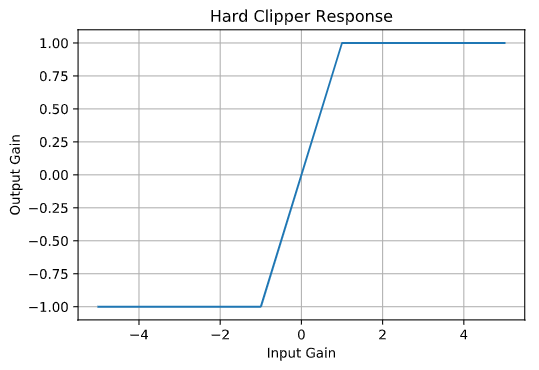
Typically, digital systems use filters to supress any signal above the Nyquist frequency, so that aliasing artifacts don’t occur. However, when using a nonlinear function, the digital system can create signal above the Nyquist frequency, thus creating aliasing artifacts. As an example let’s look at a specific type of distortion known as “hard-clipping” distortion. A hard-clipper is a waveshaping distortion with a waveshaping curve that looks as follows:

If I now create a 1.2 kHz sine wave, and process it through a hard-clipping distortion with no aliasing, I would see the following frequency response:

The spike farthest to the left represents the original sine wave, while all the other spikes represent the higher order harmonics generated by the hard-clipper. Note that all of the harmonics are evenly spaced.

Now, if we were to sample the sine wave at fs=48 kHz before processing it with the hard clipper, any generated harmonics above fs/2=24 kHz would be reflected back to produce aliasing artifacts. Let’s see what that looks like:

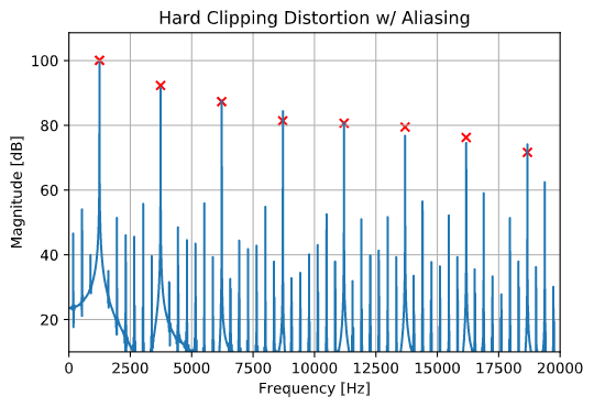
In this case, we see that all the blue spikes not marked with the red x’s are aliasing artifacts. This level of aliasing will almost certainly be audible for people listening to signals that have been processed with this effect, and probably won’t sound very pleasant.

Anti-Aliasing with Oversampling

Now that we have some understanding of what aliasing is, and how nonlinear signal processing can create aliasing, let’s look at the most common method for supressing aliasing artifacts: oversampling.

The idea behind oversampling is very simple: if we run our nonlinear process at a higher sample rate, then any harmonics produced above the Nyquist frequency can be filtered out before the audio is downsampled back to its original sample rate. Let’s see how well 4x oversampling works for out hard-clipping distortion:

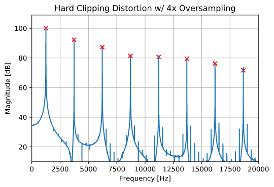
The result is pretty good! While aliasing artifacts are still visible they are at a much lower magnitude than the original signal. More oversampling can be used to supress aliasing artifacts even further.

However, using oversampling has some drawbacks, notably with performance. Specifically, the processing time for an effect will be multiplied by the oversampling factor. In other words, if a process is done with 4x oversampling, the oversampled process will be 1/4th as efficient as the original process. With that in mind, let us look for other anti-aliasing methods, that hopefully introduce less performance overhead.

Antiderivative Antialiasing

Antiderivative anti-aliasing (abbreviated as ADAA), was first introduced in a 2016 DAFx paper by Julian Parker, Vadim Zavalishin, and Efflam Le Bivic from Native Instruments. The technical background for ADAA is then further developed in an IEEE paper by Stefan Bilbao, Fabián Esqueda, Parker, and Vesa Välimäki. I won’t go to much into the mathematical details of ADAA, but the basic idea is that instead of applying a nonlinear function to a signal, we instead apply the anti-derivative of that function, and then use discrete-time differentiation resulting in a signal with supressed aliasing artifacts.

1st-order ADAA

ADAA can be implemented as follows: Say we have a nonlinear function, y[n]=f(x[n]), with an antiderivative F₁(x). A first-order ADAA version of the function, can be written as follows:

Unfortunately, when |x[n]−x[n−1]| is very small, this equation becomes ill-conditioned, similar to dividing by zero. To remedy this issue, we define a tolerance, below which |x[n]−x[n−1]| is treated as if it were zero, and then use the following equation to express first-order ADAA:

For the hard-clipper, we can write the original nonlinear function as follows:

And the first antiderivative as:

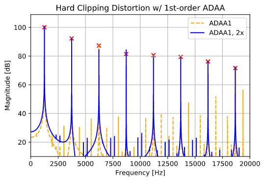
Let’s see how the aliasing artifacts look using first-order ADAA:

Clearly, the aliasing artifacts are significantly more supressed than with no anti-aliasing, however they are still of significant magnitude. One option would be to use first-order ADAA in tandem with a modest amount of oversampling, maybe 2x:

2nd-order ADAA

A second option is to use higher-order antiderivatives. Let’s say that our nonlinear function y[n]=f(x[n]) has a second antiderivative, which we’ll call F₂(x). Then second-order ADAA can be written as:

Since this equation has more divisions where a divide-by-zero error is possible, several “fallback” computations are necessary. I won’t go through them in detail here, but full derivations can be found in Stefan Bilbao’s IEEE paper (linked above), and implementations can be seen in the attached code (see below). Finally, we need the second antiderivative of our hard clipping function:

Now we can examine the response of second-order ADAA:

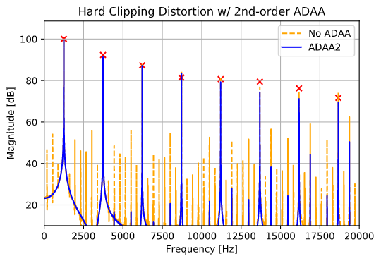
Again, using a modest amount of oversampling in conjuntion with 2nd-order ADAA can help immensly. Below, we show the response using 2x oversampling:

Tanh Distortion with ADAA

So far, we’ve only looked at using ADAA with the hard-clipping nonlinearity. Let’s move on to another nonlinear function commonly used for waveshaping distortion: the tanh function:

Let’s take a look at the frequency domain output of the tanh distortion, with and without aliasing:

In order to implement ADAA, we’ll need to find the first and second antiderivatives of f(x)=tanh(x):

Note that log(x) refers to the natural logarithm, and Li₂(x) refers to the dilogarithm function. While the dilogarithm is a tricky function to implement by hand, there are decent open-source implementations available in Python’s Scipy library, and for C/C++ in the polylogarithm library on GitHub. Note that depending on the implementation of the dilogarithm function, it may need to be called in the form Li₂(1−x).

Let’s take a look at how well first- and second-order ADAA supress aliasing artifacts for the tanh nonlinearity:

ADAA with Stateful Systems

You may have noticed that every nonlinear system examined thus far has been a “memoryless” system, i.e. the current output is dependent only on the current input, no memory of past input/output states is needed. In other systems, sometimes referred to as “stateful” systems, these past states are needed. For several years, ADAA was reputed to only work for memoryless systems, since first-order ADAA introduces 0.5 samples of group delay along the processing path. For an example of how this group delay can be problematic, let’s examine a nonlinear waveguide resonator:

The resonant frequency of the nonlinear waveguide resonator is dependent on the round-trip delay around the nonlinear feedback loop. If we were to use first-order ADAA to implement the nonlinearity, then the resonant frequency would be skewed low due to the extra half sample added to the round-trip delay time by the ADAA process. While the error in frequency might be pretty minimal (especially for low-pitched resonators, or systems with high sample rates), it can be noticeable. For example, waveguide resonators are often used to model vibrating guitar strings, an error in the frequency of the waveguide could make a guitar string go out of tune!

In this case, ADAA can be still be used, just with a small adjustment: after calculating the correct length of the delay line to use at the current sample rate, the user must subtract half a sample, to compensate for the delay added by the ADAA process.

In general, using ADAA for stateful systems can be slightly more difficult, though it is possible. For more details, see Martin Holters’ 2019 DAFx paper on the subject.

Implementation

Thus far, we’ve seen how antiderivative anti-aliasing can be useful for supressing aliasing artifacts in nonlinear systems. However, when using ADAA in practice, it can often be difficult to determine what order of ADAA is neccesary, and how it compares to using oversampling in terms of aliasing supression and computational performance. To that end, I’ve developed an audio plugin using the JUCE/C++ framework, to demonstrate the capabilities of ADAA, and allow users to find the right balance for their applications. The plugin offers three processing modes: standard, first-order ADAA, and second-order ADAA, using both real-time computation and table-lookup, as well as variable oversampling options. The idea is that users can examine what combination of ADAA and oversampling work best for their application.

Currently, I’ve implemented the hard-clipper, and tanh distortion, as well as a nonlinear waveguide, using the tanh function as the nonlinearity in the feedback path. In the future, I hope to add more nonlinear systems, such as nonlinear filters, and wave digital filters (inspired by Davide Albertini’s recent paper). The project is open-source, so if you have a nonlinear system you’d like to see included, feel free to code it up for yourself!

Source code and further documentation can be found on GitHub.

Acknowledgements

Big thanks to Matt Nielsen for inspiring this project, and for some insightful conversations!